Structure factor

Class collecting estimators of the structure factor $S(\mathbf{k})$ of stationary point process given one realization encapsulated in a PointPattern.

The available estimators:

scattering_intensity(): The scattering intensity and the corresponding debiased versions.
tapered_estimator(): The tapered or multitapered estimator and the corresponding debiased versions.
tapered_estimator_isotropic(): Bartlett’s isotropic estimator.
quadrature_estimator_isotropic(): Integral estimation using Hankel transform quadrature.

The available plot methods:

plot_non_isotropic_estimator(): Visualize the results of scattering_intensity(), tapered_estimator(), or multitapered_estimator().
plot_isotropic_estimator(): Visualize the results of tapered_estimator_isotropic() or quadrature_estimator_isotropic().

For the theoretical derivation and definitions of these estimators, we refer to [HGBLachiezeR22].

class structure_factor.structure_factor.StructureFactor(point_pattern)[source]

Bases: object

Implementation of various estimators of the structure factor $S(\mathbf{k})$ of a stationary point process given one realization encapsulated in the point_pattern attribute.

Definition

The structure factor $S$ of a d-dimensional stationary point process $\mathcal{X}$ with intensity $\rho$ is defined by,

\[S(\mathbf{k}) = 1 + \rho \mathcal{F}(g-1)(\mathbf{k}),\]

where $\mathcal{F}$ denotes the Fourier transform, $g$ the pair correlation function of $\mathcal{X}$, $\mathbf{k}$ a wavevector of $\mathbb{R}^d$. For more details we refer to [HGBLachiezeR22], (Section 2) or [Tor18], (Section 2.1, equation (13)).

__init__(point_pattern)[source]

Initialize StructureFactor from point_pattern.

Parameters: point_pattern (PointPattern) – Object of type point pattern which contains a realization point_pattern.points of a point process, the window where the points were simulated point_pattern.window and (optionally) the intensity of the point process point_pattern.intensity.

property dimension: Ambient dimension of the underlying point process.

scattering_intensity(k=None, debiased=True, direct=True, **params)[source]

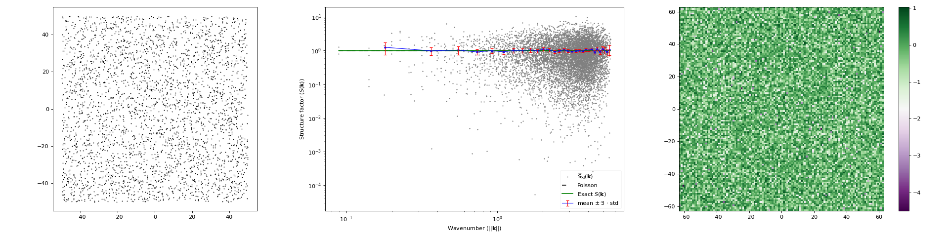
Compute the scattering intensity $\widehat{S}_{\mathrm{SI}}$ estimate of the structure factor from one realization of a stationary point process encapsulated in the point_pattern attribute.

Parameters

k (numpy.ndarray, optional) – Array of size $n \times d$ where $d$ is the dimension of the space, and $n$ is the number of wavevectors where the scattering intensity is evaluated. If k=None and debiased=True, the scattering intensity will be evaluated on the corresponding set of allowed wavevectors; In this case, the keyword arguments k_max, and meshgrid_shape can be used. Defaults to None.
debiased (bool, optional) –
Trigger the use of a debiased tapered estimator. Defaults to True. If debiased=True, the estimator is debiased as follows,
- if k=None, the scattering intensity will be evaluated on the corresponding set of allowed wavevectors.
- if k is not None and direct=True, the direct debiased scattering intensity will be used,
- if k is not None and direct=False, the undirect debiased scattering intensity will be used.
direct (bool, optional) – If debiased is True, trigger the use of the direct/undirect debiased scattering intensity. Parameter related to debiased. Defaults to True.

Keyword Arguments

params (dict) – Keyword arguments k_max and meshgrid_shape of allowed_k_scattering_intensity(), used when k=None and debiased=True.

Returns

k: Wavevector(s) on which the scattering intensity has been evaluated.
estimation: Evaluation of the scattering intensity estimator of the structure factor at k.

Return type

tuple(numpy.ndarray, numpy.ndarray)

Example

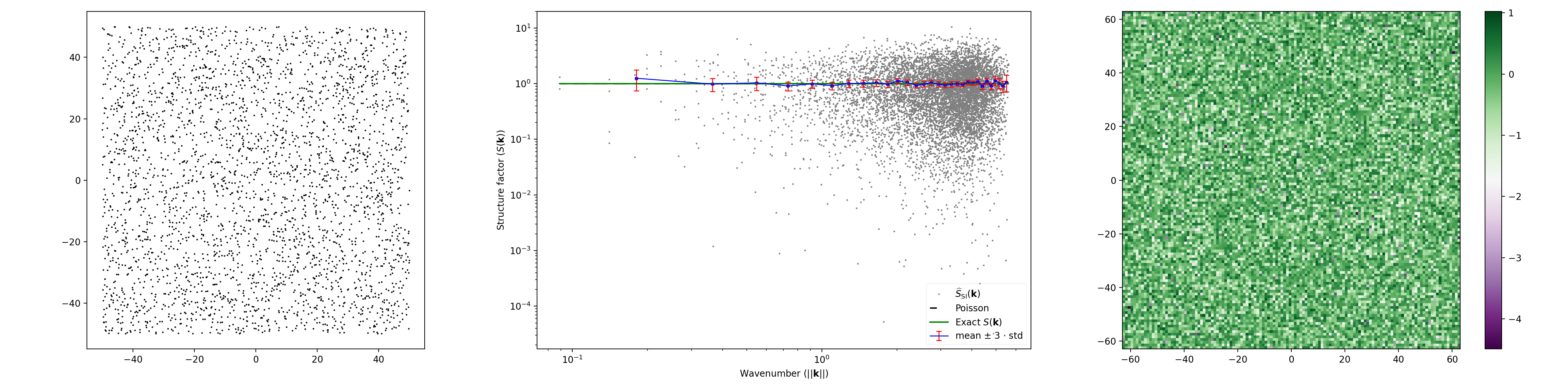
import matplotlib.pyplot as plt
import numpy as np

from structure_factor.point_processes import HomogeneousPoissonPointProcess
from structure_factor.spatial_windows import BoxWindow
from structure_factor.structure_factor import StructureFactor

point_process = HomogeneousPoissonPointProcess(intensity=1 / np.pi)

window = BoxWindow([[-50, 50], [-50, 50]])
point_pattern = point_process.generate_point_pattern(window=window)

sf = StructureFactor(point_pattern)
k, sf_estimated = sf.scattering_intensity(k_max=4)

sf.plot_non_isotropic_estimator(
    k,
    sf_estimated,
    plot_type="all",
    error_bar=True,
    bins=30,
    exact_sf=point_process.structure_factor,
    scale="log",
    label=r"$\widehat{S}_{\mathrm{SI}}(\mathbf{k})$",
)

plt.tight_layout(pad=1)

(Source code, png, hires.png, pdf)

Definition

The scattering intensity $\widehat{S}_{\mathrm{SI}}$ is an estimator of the structure factor $S$ of a stationary point process $\mathcal{X} \subset \mathbb{R}^d$ with intensity $\rho$. It is computed from one realization $\mathcal{X}\cap W =\{\mathbf{x}_i\}_{i=1}^N$ of $\mathcal{X}$ within a box window $W=\prod_{j=1}^d[-L_j/2, L_j/2]$.

\[\widehat{S}_{\mathrm{SI}}(\mathbf{k}) = \frac{1}{N}\left\lvert \sum_{j=1}^N \exp(- i \left\langle \mathbf{k}, \mathbf{x_j} \right\rangle) \right\rvert^2 .\]

For more details we refer to [HGBLachiezeR22], (Section 3.1).

Note

Typical usage

If the observation window is not a BoxWindow, use the method restrict_to_window() to extract a sub-sample in a BoxWindow.

See also

tapered_estimator(k, tapers, debiased=True, direct=True)[source]

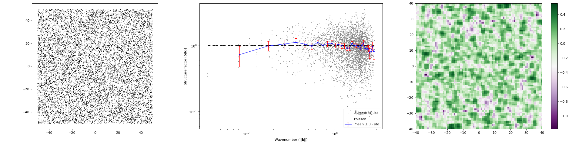
Compute the (multi)tapered estimator parametrized by tapers of the structure factor of a stationary point process given a realization encapsulated in point_pattern.

Parameters

k (numpy.ndarray) – Array of size $n \times d$ where $d$ is the dimension of the space, and $n$ is the number of wavevectors where the tapered estimator is evaluated.
t1 – sequence of concrete tapers with methods .taper(x, window) corresponding to the taper function $t(x, W)$ , and .ft_taper(k, window) corresponding to the Fourier transform $\mathcal{F}[t(\cdot, W)](k)$ of the taper. See also Tapers.
t2 – sequence of concrete tapers with methods .taper(x, window) corresponding to the taper function $t(x, W)$ , and .ft_taper(k, window) corresponding to the Fourier transform $\mathcal{F}[t(\cdot, W)](k)$ of the taper. See also Tapers.
... – sequence of concrete tapers with methods .taper(x, window) corresponding to the taper function $t(x, W)$ , and .ft_taper(k, window) corresponding to the Fourier transform $\mathcal{F}[t(\cdot, W)](k)$ of the taper. See also Tapers.
debiased (bool, optional) – Trigger the use of a debiased estimator. Defaults to True.
direct (bool, optional) – If debiased is True, trigger the use of the direct/undirect debiased tapered estimator. Parameter related to debiased. Defaults to True.

Returns

k: Wavevector(s) on which the tapered estimator has been evaluated.
estimation: Evaluation of the tapered estimator at k..

Return type

tuple(numpy.ndarray, numpy.ndarray)

Note

Calling this method with its default arguments is equivalent to calling scattering_intensity().

Example

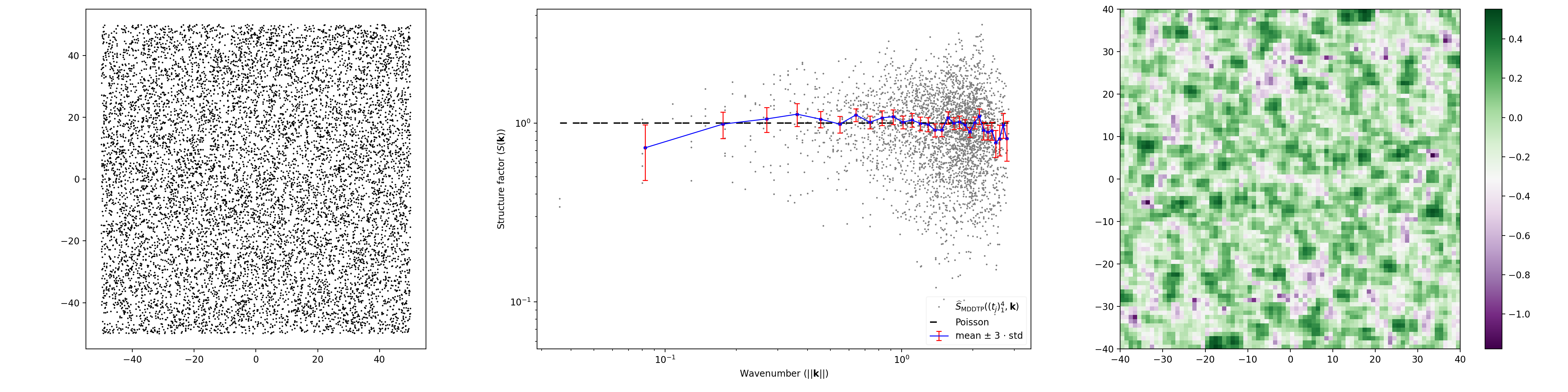
import matplotlib.pyplot as plt
import numpy as np

from structure_factor.point_processes import HomogeneousPoissonPointProcess
from structure_factor.spatial_windows import BoxWindow
from structure_factor.structure_factor import StructureFactor
from structure_factor.tapers import multi_sinetaper_grid
from structure_factor.utils import meshgrid_to_column_matrix

point_process = HomogeneousPoissonPointProcess(intensity=1)
window = BoxWindow([[-50, 50], [-50, 50]])
point_pattern = point_process.generate_point_pattern(window=window)

sf = StructureFactor(point_pattern)

# Use the family of sine tapers
x = np.linspace(-2, 2, 80)
x = x[x != 0]
k = meshgrid_to_column_matrix(np.meshgrid(x, x))


tapers = multi_sinetaper_grid(point_pattern.dimension, p_component_max=2)
k, sf_estimated = sf.tapered_estimator(k, tapers=tapers, debiased=True, direct=True)

sf.plot_non_isotropic_estimator(
    k,
    sf_estimated,
    plot_type="all",
    error_bar=True,
    bins=30,
    label=r"$\widehat{S}_{\mathrm{MDDTP}}((t_j)_1^4, \mathbf{k})$",
)

plt.tight_layout(pad=1)

(Source code, png, hires.png, pdf)

Definition

The tapered estimator $\widehat{S}_{\mathrm{TP}}(t, k)$, is an estimator of the structure factor $S$ of a stationary point process $\mathcal{X} \subset \mathbb{R}^d$ with intensity $\rho$. It is computed from one realization $\mathcal{X}\cap W =\{\mathbf{x}_i\}_{i=1}^N$ of $\mathcal{X}$ within a box window $W$.

\[\widehat{S}_{\mathrm{TP}}(t, \mathbf{k}) = \frac{1}{\rho} \left\lvert \sum_{j=1}^N t(x_j, W) \exp(- i \left\langle k, x_j \right\rangle)\right\rvert^2,\]

If several tapers are used, a simple average of the corresponding tapered estimators is computed. The resulting estimator is call multitapered estimator.

\[\widehat{S}_{\mathrm{MTP}}((t_{q})_{q=1}^P, \mathbf{k}) = \frac{1}{P}\sum_{q=1}^{P} \widehat{S}(t_{q}, \mathbf{k})\]

where, $(t_{q})_{q}$ is a family of tapers supported on the observation window (satisfying some conditions), $P$ is the number of tapers used, and $k \in \mathbb{R}^d$. For more details, we refer to [HGBLachiezeR22], (Section 3.1).

Note

Typical usage

If the observation window is not a BoxWindow, use the method restrict_to_window() to extract a sub-sample in a BoxWindow.

See also

bartlett_isotropic_estimator(k_norm=None, **params)[source]

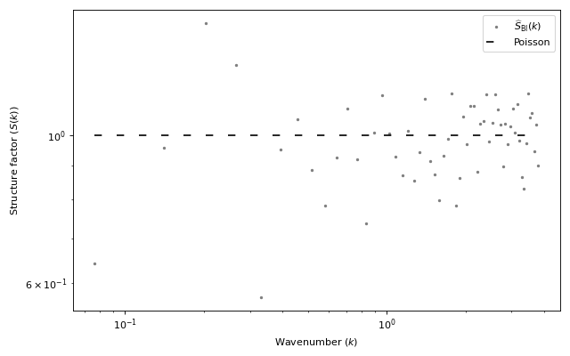
Compute Bartlett’s isotropic estimator $\widehat{S}_{\mathrm{BI}}$ from one realization of an isotropic point process encapsulated in the point_pattern attribute.

Parameters

k_norm (numpy.ndarray, optional) – Array of wavenumbers of size $n$ where the estimator is to be evaluated. Defaults to None.

Keyword Arguments

params (dict) – Keyword argument nb_values of allowed_k_norm_bartlett_isotropic used when ``k_norm=None`() to specify the number of allowed wavenumbers to be considered.

Returns

k_norm: Wavenumber(s) on which Bartlett’s isotropic estimator has been evaluated.
estimation: Evaluation(s) of Bartlett’s isotropic estimator at k.

Return type

tuple(numpy.ndarray, numpy.ndarray)

Example

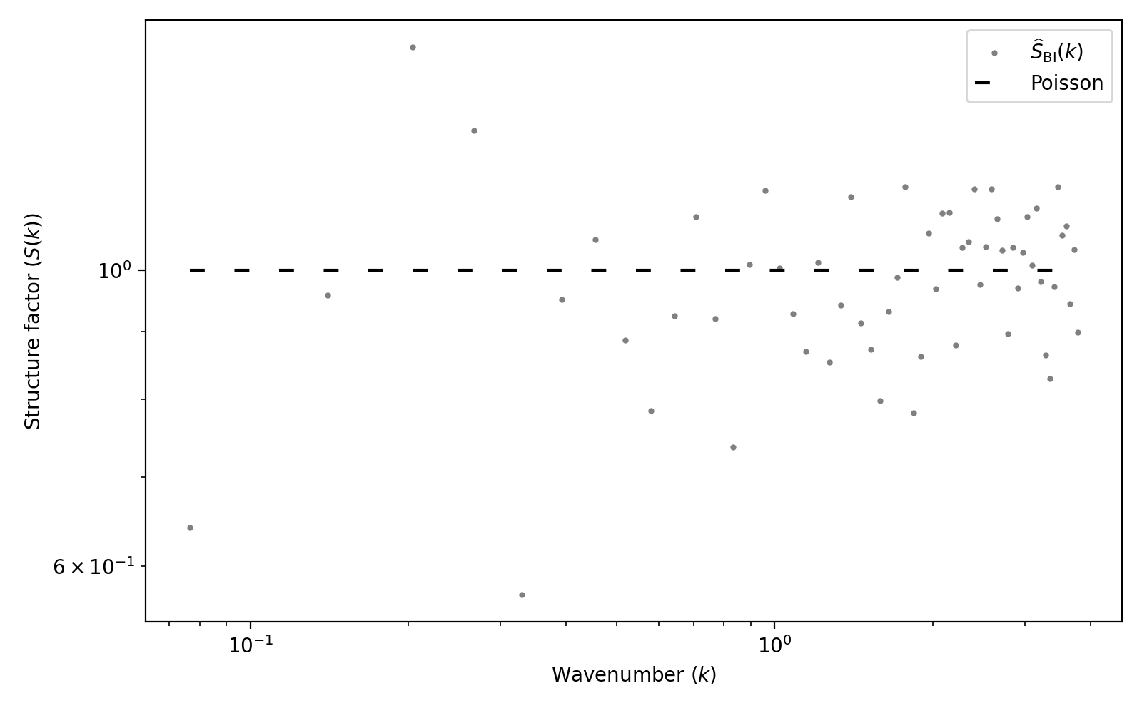
import matplotlib.pyplot as plt

from structure_factor.point_processes import HomogeneousPoissonPointProcess
from structure_factor.spatial_windows import BallWindow
from structure_factor.structure_factor import StructureFactor
from structure_factor.tapered_estimators_isotropic import (
    allowed_k_norm_bartlett_isotropic,
)

point_process = HomogeneousPoissonPointProcess(intensity=1)
window = BallWindow(center=[0, 0], radius=50)
point_pattern = point_process.generate_point_pattern(window=window)

sf = StructureFactor(point_pattern)
d, r = point_pattern.dimension, point_pattern.window.radius
k_norm = allowed_k_norm_bartlett_isotropic(dimension=d, radius=r, nb_values=60)
k_norm, sf_estimated = sf.bartlett_isotropic_estimator(k_norm)

ax = sf.plot_isotropic_estimator(
    k_norm, sf_estimated, label=r"$\widehat{S}_{\mathrm{BI}}(k)$"
)

plt.tight_layout(pad=1)

(Source code, png, hires.png, pdf)

_images/bartlett_isotropic_estimator.png

Definition

Bartlett’s isotropic estimator $\widehat{S}_{\mathrm{BI}}$ is an estimator of the structure factor $S$ of a stationary isotropic point process $\mathcal{X} \subset \mathbb{R}^d$ with intensity $\rho$. It is computed from one realization $\mathcal{X}\cap W =\{\mathbf{x}_i\}_{i=1}^N$ of $\mathcal{X}$ within a ball window $W=B(\mathbf{0}, R)$.

\[\begin{split}\widehat{S}_{\mathrm{BI}}(k) = 1 + \frac{ (2\pi)^{d/2} }{\rho |W| \omega_{d-1}} \sum_{ \substack{j, q =1 \\ j\neq q } }^{N } \frac{1}{(k \|\mathbf{x}_j - \mathbf{x}_q\|_2)^{d/2 - 1}} J_{d/2 - 1}(k \|\mathbf{x}_j - \mathbf{x}_q\|_2).\end{split}\]

For more details, we refer to [HGBLachiezeR22], (Section 3.2).

Note

Typical usage

If the observation window is not a BallWindow, use the method restrict_to_window() to extract a sub-sample in a BallWindow.

See also

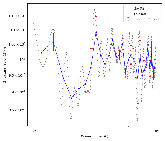
quadrature_estimator_isotropic(pcf, k_norm=None, method='BaddourChouinard', **params)[source]

Approximate the structure factor of a stationary isotropic point process at values k_norm, given its pair correlation function pcf, using a quadrature method.

Warning

It only applies to point processes in even dimension $d$, due to evaluations of the zeros of Bessel functions of order $d / 2 - 1$ that must integer-valued.

Parameters

pcf (callable) – Pair correlation function.
k_norm (numpy.ndarray, optional) – Vector of wavenumbers (i.e., norms of wavevectors) where the structure factor is to be evaluated. Optional if method="BaddourChouinard" (since this method evaluates the Hankel transform on a specific set of wavenumbers), but it is non optional if method="Ogata". Defaults to None.
method (str, optional) –
Trigger the use of "BaddourChouinard" or "Ogata" quadrature to estimate the structure factor. Defaults to "BaddourChouinard",
- if "BaddourChouinard": The Hankel transform is approximated using the Discrete Hankel transform [BC15]. See HankelTransformBaddourChouinard
- if "Ogata": The Hankel transform is approximated using Ogata quadrature [Oga05]. See HankelTransformOgata

Keyword Arguments

params (dict) –

Keyword arguments passed to the corresponding Hankel transformer selected according to the input argument method.

method == "Ogata", see compute_transformation_parameters()
- step_size
- nb_points
method == "BaddourChouinard", see compute_transformation_parameters()
- r_max
- nb_points
- interpolotation dictionnary containing the keyword arguments of scipy.integrate.interp1d parameters.

Returns

k_norm: Vector of wavenumbers.
estimation: Evaluations of the structure factor on k_norm.

Return type

tuple (numpy.ndarray, numpy.ndarray)

Example

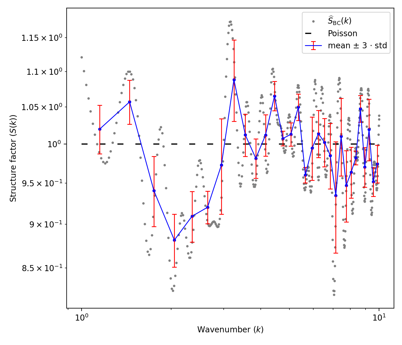
import matplotlib.pyplot as plt
import numpy as np

import structure_factor.pair_correlation_function as pcf
from structure_factor.point_processes import HomogeneousPoissonPointProcess
from structure_factor.spatial_windows import BallWindow
from structure_factor.structure_factor import StructureFactor

point_process = HomogeneousPoissonPointProcess(intensity=1)

window = BallWindow(center=[0, 0], radius=40)
point_pattern = point_process.generate_point_pattern(window=window)

pcf_estimated = pcf.estimate(
    point_pattern, method="fv", Kest=dict(rmax=20), fv=dict(method="c", spar=0.2)
)

# Interpolate/extrapolate the results
r = pcf_estimated["r"]
pcf_r = pcf_estimated["pcf"]
pcf_interpolated = pcf.interpolate(r=r, pcf_r=pcf_r, drop=True)

# Estimate the structure factor using Baddour Chouinard quadrature
sf = StructureFactor(point_pattern)
k_norm = np.linspace(1, 10, 500)  # vector of wavelength
k_norm, sf_estimated = sf.quadrature_estimator_isotropic(
    pcf_interpolated, method="BaddourChouinard", k_norm=k_norm, r_max=20, nb_points=1000
)

fig, ax = plt.subplots(figsize=(7, 6))
fig = sf.plot_isotropic_estimator(
    k_norm,
    sf_estimated,
    axis=ax,
    error_bar=True,
    bins=30,
    label=r"$\widehat{S}_{\mathrm{BC}}(k)$",
)
plt.tight_layout(pad=1)

(Source code, png, hires.png, pdf)

Definition

The structure factor $S$ of a stationary isotropic point process $\mathcal{X} \subset \mathbb{R}^d$ with intensity $\rho$, can be defined via the Hankel transform $\mathcal{H}_{d/2 -1}$ of order $d/2 -1$ as follows,

\[S(\|\mathbf{k}\|_2) = 1 + \rho \frac{(2 \pi)^{d/2}}{\|\mathbf{k}\|_2^{d/2 -1}} \mathcal{H}_{d/2 -1}(\tilde g -1)(\|\mathbf{k}\|_2), \quad \tilde g: x \mapsto g(x) x^{d/2 -1},\]

where, $g$ is the pair correlation function of $\mathcal{X}$.

This is a result of the relation between the Symmetric Fourier transform and the Hankel Transform. For more details, we refer to [HGBLachiezeR22], (Section 3.2).

Note

Typical usage

Estimate the pair correlation function using estimate().

Clean and interpolate/extrapolate the resulting estimation using interpolate() to get a function.

Use the result as the input pcf.

See also

plot_isotropic_estimator(k_norm, estimation, axis=None, scale='log', k_norm_min=None, exact_sf=None, color='grey', error_bar=False, label='$\\widehat{S}$', file_name='', **binning_params)[source]

Display the outputs of the method quadrature_estimator_isotropic(), or tapered_estimator_isotropic().

Parameters

k_norm (numpy.ndarray) – Vector of wavenumbers (i.e., norms of wavevectors) on which the structure factor has been approximated.
estimation (numpy.ndarray) – Approximation(s) of the structure factor corresponding to k_norm.
axis (plt.Axes, optional) – Support axis of the plot. Defaults to None.
scale (str, optional) – Trigger between plot scales of see matplolib documentation. Defaults to ‘log’.
k_norm_min (float, optional) – Estimated lower bound of the wavenumbers. Defaults to None.
exact_sf (callable, optional) – Theoretical structure factor of the point process. Defaults to None.
error_bar (bool, optional) – If True, k_norm and correspondingly estimation, are divided into sub-intervals (bins). Over each bin, the mean and the standard deviation of si are derived and visualized on the plot. Note that each error bar corresponds to the mean $\pm 3 \times$ standard deviation. To specify the number of bins, add it as a keyword argument. For more details see _bin_statistics(). Defaults to False.
file_name (str, optional) – Name used to save the figure. The available output formats depend on the backend being used. Defaults to “”.

Keyword Arguments

binning_params – (dict): Used when error_bar=True, by the method utils_bin_statistics() as keyword arguments (except "statistic") of scipy.stats.binned_statistic.

Returns

Plot of the approximated structure factor.

Return type

plt.Axes

plot_non_isotropic_estimator(k, estimation, axes=None, scale='log', plot_type='radial', positive=False, exact_sf=None, error_bar=False, label='$\\widehat{S}$', rasterized=True, file_name='', window_res=None, **binning_params)[source]

Display the outputs of the method scattering_intensity(), tapered_estimator().

Parameters

k (numpy.ndarray) – Wavevector(s) on which the scattering intensity has been approximated. Array of size $n \times d$ where $d$ is the dimension of the space, and $n$ is the number of wavevectors.
estimation (numpy.ndarray) – Approximated structure factor associated to k.
axes (plt.Axes, optional) – Support axes of the plots. Defaults to None.
scale (str, optional) –
Trigger between plot scales of see matplolib documentation. Defaults to “log”.
plot_type (str, optional) –
Type of the plot to visualize, “radial”, “imshow”, or “all”. Defaults to “radial”.
- If “radial”, the output is a 1D plot of estimation w.r.t. the norm(s) of k.
- If “imshow” (option available only for a 2D point process), the output is a 2D color level plot.
- If “all” (option available only for a 2D point process), the result contains 3 subplots: the point pattern (or a restriction to a specific window if window_res is set), the radial plot, and the color level plot. Note that the options “imshow” and “all” couldn’t be used, if k couldn’t be reshaped as a meshgrid.
positive (bool, optional) – If True, consider only the positive values of estimation. Defaults to False.
exact_sf (callable, optional) – Theoretical structure factor of the point process. Defaults to None.
error_bar (bool, optional) – If True, k_norm and correspondingly estimation, are divided into sub-intervals (bins). Over each bin, the mean and the standard deviation of estimation are derived and visualized on the plot. Note that each error bar corresponds to the mean $\pm 3 \times$ standard deviation. To specify the number of bins, add it as a keyword argument. For more details see _bin_statistics(). Defaults to False.
rasterized (bool, optional) – Rasterized option of matlplotlib.plot. Defaults to True.
file_name (str, optional) – Name used to save the figure. The available output formats depend on the backend being used. Defaults to “”.
window_res (AbstractSpatialWindow, optional) – New restriction window. Useful when the sample of points is large and “plt_type=’all’”, so for time and visualization purposes, it is better to restrict the plot of the point process to a smaller window. Defaults to None.

Keyword Arguments

binning_params (dict) –

Used when error_bar=True, by the method _bin_statistics() as keyword arguments (except "statistic") of scipy.stats.binned_statistic.

Returns

Plot of the approximated structure factor.

Return type

plt.Axes