Hyperuniformity

Functions designed to study the hyperuniformity of a stationary point process using estimation(s) of its structure factor StructureFactor.

Hyperuniformity diagnostics:

multiscale_test(): Statistical test of hyperuniformity asymptomatically valid.

effective_hyperuniformity(): Test of effective hyperuniformity.

hyperuniformity_class(): Estimation of the possible class of hyperuniformity.

Additional functions:

bin_data(): Method for regularizing structure factor’s estimation.
subwindows(): Method for generating a list of subwindows from a father window with the corresponding minimum allowed wavevectors (or wavenumbers).

Note

Typical usage

Test the hyperuniformity using the statistical test multiscale_test() or the test of effective hyperuniformity effective_hyperuniformity().
If the hyperuniformity was approved, find the possible hyperuniformity class using hyperuniformity_class().

structure_factor.hyperuniformity.multiscale_test(point_pattern_list, estimator, subwindows_list, k_list, mean_poisson, m_list=None, proba_list=None, verbose=False, **kwargs)[source]

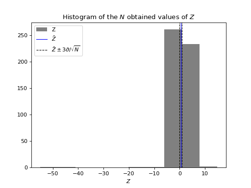
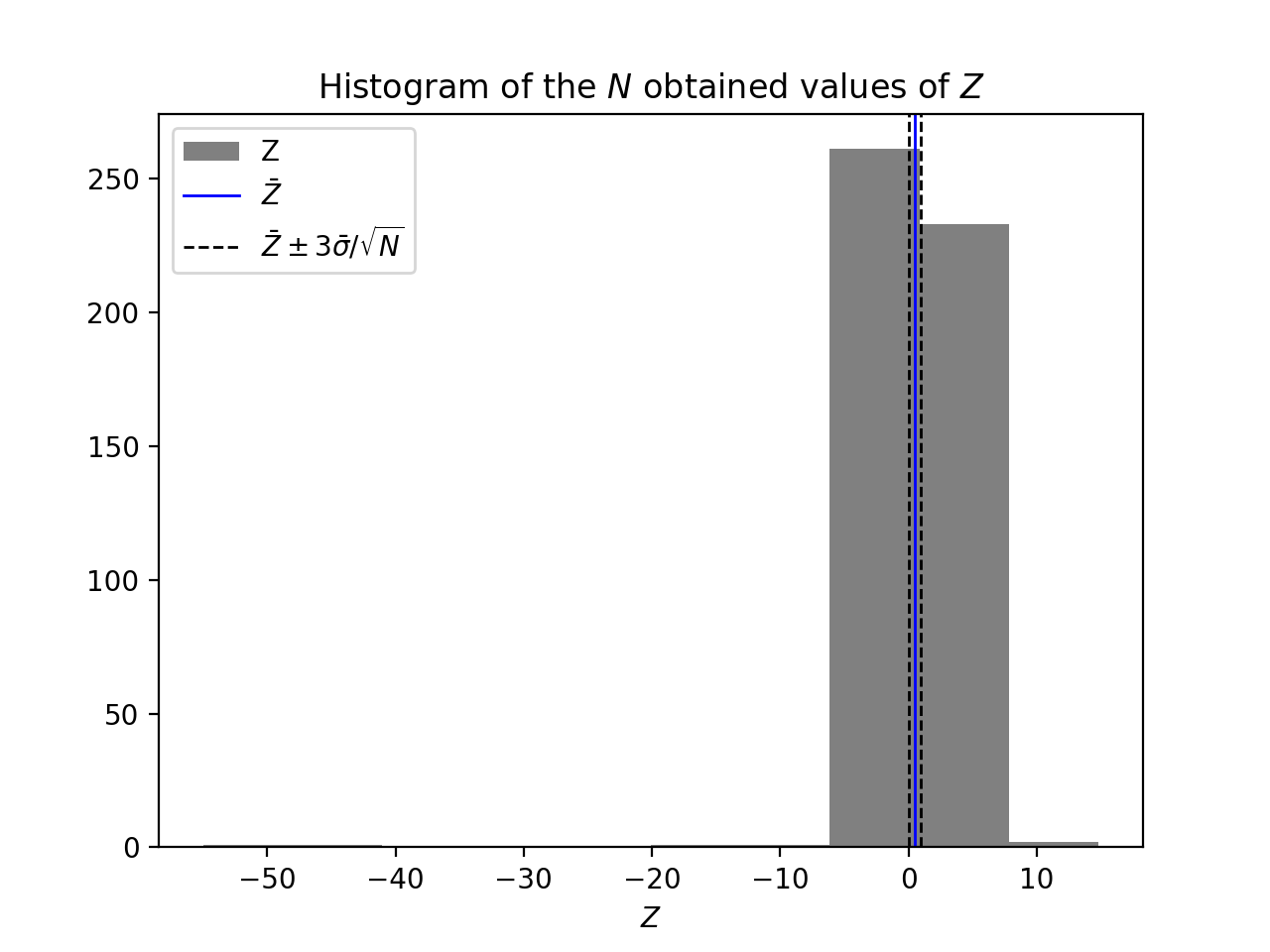
Compute the sample mean \(\bar{Z}\) and the corresponding standard deviation \(\bar{\sigma}/\sqrt{N}\) of the coupled sum estimator \(Z\) of a point process using a list of \(N\) PointPatterns and \(N\) realizations from the random variable \(M\).

The test rejects the hyperuniformity hypothesis if the confidence interval \(CI[\mathbb{E}[Z]]= [\bar{Z} - z \bar{\sigma}/\sqrt{N}, \bar{Z} + z \bar{\sigma}/\sqrt{N}]\), doesn’t contain zero, and vice-versa. (See the multiscale hyperuniformity test in [HGBLachiezeR22]).

Parameters

point_pattern_list (list) – List of PointPattern (s). Each element of the list is an encapsulation of a realization of a point process, the observation window, and (optionally) the intensity of the point process. All PointPattern (s) should have the same window and intensity.
estimator (str) – Choice of structure factor’s estimator. The parameters of the chosen estimator must be added as keyword arguments. The available estimators are “scattering_intensity”, “tapered_estimator”, “bartlett_isotropic_estimator”, and “quadrature_estimator_isotropic”. See StructureFactor.
subwindows_list (list) – List of increasing cubic or ball-shaped AbstractSpatialWindow, typically, obtained using subwindows(). The shape of the windows depends on the choice of the estimator. Each element of point_pattern_list will be restricted to these windows to compute \(Z\).
k_list (list) – List of wavevectors (or wavenumbers) where the estimator is to be evaluated. Each element is associated with an element of subwindows_list. Typically, obtained using subwindows().
mean_poisson (int) – Parameter of the Poisson r.v. \(M\) used to compute \(Z\). To use a different distribution of the r.v. \(M\), set mean_poisson=None and specify m_list and proba_list corresponding to \(M\).
m_list (list, optional) – List of positive integer realizations of the r.v. \(M\), used when mean_poisson=None. Each element of m_list is associated with an element of point_pattern_list to compute a realization of \(Z\). Defaults to None.
proba_list (list, optional) – List of \(\mathbb{P}(M \geq j)\) used with m_list when mean_poisson=None. Should contains at least max(m_list) elements. Defaults to None.
verbose (bool, optional) – If “True” and mean_poisson is not None, print the re-sampled values of \(M\). Defaults to False.

Keyword Arguments

kwargs (dict) – Parameters of the chosen estimator of the structure factor. See StructureFactor.

Returns

“mean_Z”: The sample mean of \(Z\).
”std_mean_Z”: The sample standard deviation of \(Z\) divided by the square root of the number of samples.
”Z”: The obtained values of \(Z\).
”M”: The used values of \(M\).

Return type

dict(float, float, list, list)

Example

import numpy as np
from structure_factor.point_processes import HomogeneousPoissonPointProcess
from structure_factor.spatial_windows import BoxWindow
from structure_factor.hyperuniformity import subwindows, multiscale_test

# PointPattern list
poisson = HomogeneousPoissonPointProcess(intensity=1 / np.pi)
N = 500
L = 160
window = BoxWindow([[-L / 2, L / 2]] * 2)
point_patterns = [
    poisson.generate_point_pattern(window=window) for _ in range(N)
]
# subwindows and k
l_0 = 40
subwindows_list, k = subwindows(window, subwindows_type="BoxWindow", param_0=l_0)

# multiscale hyperuniformity test
mean_poisson = 90
summary = multiscale_test(point_patterns,
    estimator="scattering_intensity", k_list=k,
    subwindows_list=subwindows_list, mean_poisson=mean_poisson,
    verbose=True)

import matplotlib.pyplot as plt
plt.hist(summary["Z"], color="grey", label="Z")
plt.axvline(summary["mean_Z"], color="b", linewidth=1, label=r"$\bar{Z}$")
plt.axvline(summary["mean_Z"] - 3*summary["std_mean_Z"], linestyle='dashed',
            color="k", linewidth=1, label=r"$\bar{Z} \pm 3 \bar{\sigma}/ \sqrt{N}$")
plt.axvline(summary["mean_Z"] + 3*summary["std_mean_Z"], linestyle='dashed',
            color="k", linewidth=1)
plt.xlabel(r"$Z$")
plt.title(r"Histogram of the $N$ obtained values of $Z$")
plt.legend()
plt.show()

(Source code, png, hires.png, pdf)

Definition

Let \(\mathcal{X} \in \mathbb{R}^d\) be a stationary point process of which we consider an increasing sequence of sets \((\mathcal{X} \cap W_m)_{m \geq 1}\), with \((W_m)_m\) centered box (or ball)-shaped windows s.t. \(W_s \subset W_r\) for all \(0< s<r\), and \(W_{\infty} = \mathbb{R}^d\). We define the sequence of r.v. \(Y_m = 1\wedge \widehat{S}_m(\mathbf{k}_m^{\text{min}})\), where \(\widehat{S}_m\) is one of the positive, asymptotically unbiased estimators of the structure factor of \(\mathcal{X}\) applied on the observation \(\mathcal{X} \cap W_m\), and \(\mathbf{k}_m^{\text{min}}\) is the minimum allowed wavevector associated with \(W_m\).

Under some assumptions ([HGBLachiezeR22], Section 4) \(\mathcal{X}\) is hyperuniform iff \(\mathbb{E}[Z]=0\). Where \(Z\) is the coupled sum estimator of [RG15] defined by,

\[Z = \sum_{j=1}^{M} \frac{Y_j - Y_{j-1}}{\mathbb{P}(M\geq j)},\]

with \(M\) an \(\mathbb{N}\)-valued random variable such that \(\mathbb{P}(M \geq j)>0\) for all \(j\), and \(Y_{0}=0\).

Important

If mean_poisson is not None, there is a step of accepting/rejecting while sampling from the r.v. \(M\). If the biggest subwindow associated with \(M'\) (obtained value of \(M\)) is larger than the father window, then \(M'\) is rejected, and we resample from \(M\). Typically, mean_poisson should be chosen s.t. the probability that the biggest subwindow is larger than the father window is small enough.
The test is asymptotically valid, so it might fail in diagnosing hyperuniformity if the number of samples used to compute \(\bar{Z}\) or \(\lambda\) is too small.

Note

Typical usage

The function subwindows() can be used to generate from a father window a list of subwindows and the associated allowed wavevectors/wavenumbers.

See also

structure_factor.hyperuniformity.effective_hyperuniformity(k_norm, sf, k_norm_stop, std_sf=None, **kwargs)[source]

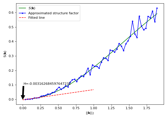
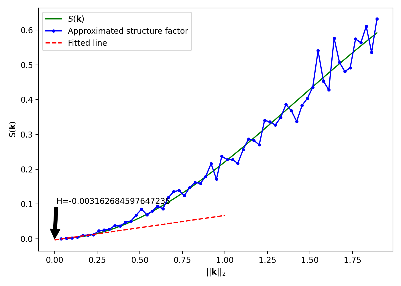
Evaluate the index \(H\) of hyperuniformity of a point process using its structure factor sf. If \(H<10^{-3}\) the corresponding point process is deemed effectively hyperuniform.

Parameters

k_norm (numpy.ndarray) – Vector of wavenumbers (i.e. norms of wavevectors).
sf (numpy.ndarray) – Evaluations of the structure factor, of the given point process, at k_norm.
std_sf (numpy.ndarray, optional) – Standard deviations associated with sf. Defaults to None.
k_norm_stop (float) – Threshold on k_norm. Used to find the numerator of \(H\) by linear regression of sf up to the value associated with k_norm_stop.

Keyword Arguments

kwargs (dict) – Keyword arguments (except “sigma”) of scipy.scipy.optimize.curve_fit parameters.

Returns

“H”: Value of the index \(H\).
”s0_std”: Standard deviation of the numerator of \(H\).
”fitted_line”: Line used to find the numerator of \(H\).
”idx_first_peak”: Index of \(k_{peak}\) if it exists.

Return type

dict(float, float, function, int)

Example

import matplotlib.pyplot as plt
import numpy as np
from structure_factor.data import load_data
from structure_factor.hyperuniformity import effective_hyperuniformity
from structure_factor.point_processes import GinibrePointProcess
from structure_factor.structure_factor import StructureFactor
from structure_factor.tapered_estimators_isotropic import (
    allowed_k_norm_bartlett_isotropic,
)

point_pattern = load_data.load_ginibre()
point_process = GinibrePointProcess()

sf = StructureFactor(point_pattern)
d, r = point_pattern.dimension, point_pattern.window.radius
k_norm = allowed_k_norm_bartlett_isotropic(dimension=d, radius=r, nb_values=60)
k_norm, sf_estimated = sf.bartlett_isotropic_estimator(k_norm)

summary = effective_hyperuniformity(k_norm, sf_estimated, k_norm_stop=0.2)
x = np.linspace(0, 1, 300)
sf_fitted_line = summary["fitted_line"](x)

sf_theoretical = point_process.structure_factor(k_norm)
fig, ax = plt.subplots(figsize=(7, 5))
ax.plot(k_norm, sf_theoretical, "g", label=r"$S(\mathbf{k})$")
ax.plot(k_norm, sf_estimated, "b", marker=".", label="Approximated structure factor")
ax.plot(x, sf_fitted_line, "r--", label="Fitted line")

ax.annotate(
    "H={}".format(summary["H"]),
    xy=(0, 0),
    xytext=(0.01, 0.1),
    arrowprops=dict(facecolor="black", shrink=0.0001),
)
ax.legend()
ax.set_xlabel(r"$||\mathbf{k}||_2$")
ax.set_ylabel(r"$\mathsf{S}(\mathbf{k})$")
plt.tight_layout(pad=1)

(Source code, png, hires.png, pdf)

Definition

A stationary isotropic point process \(\mathcal{X} \subset \mathbb{R}^d\), is said to be effectively hyperuniform if \(H \leq 10^{-3}\) where \(H\) is defined following [Tor18] (Section 11.1.6) and [KLovricC+19] (supplementary Section 8) by,

\[H = \frac{\hat{S}(\mathbf{0})}{S(\mathbf{k}_{peak})}\cdot\]

\(S\) is the structure factor of \(\mathcal{X}\),
\(\hat{S}(\mathbf{0})\) is a linear extrapolation of the structure factor at \(\mathbf{k}=\mathbf{0}\),
\(\mathbf{k}_{peak}\) is the location of the first dominant peak value of \(S\).

For more details, we refer to [HGBLachiezeR22] (Section 2.5).

Important

To compute \(\hat{S}(\mathbf{0})\), a linear extrapolation with a least-square fit is used to fit a line on the values of sf associated with a subvector of k_norm. This subvector is obtained by truncating k_norm around k_norm_stop. For the choice of k_norm_stop, the trade-off is to remain close to zero while including enough data points to fit a line. In addition, std_sf will be considered while fitting the line if it’s not None.

See also

StructureFactor
bin_data()
hyperuniformity_class()

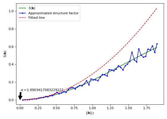
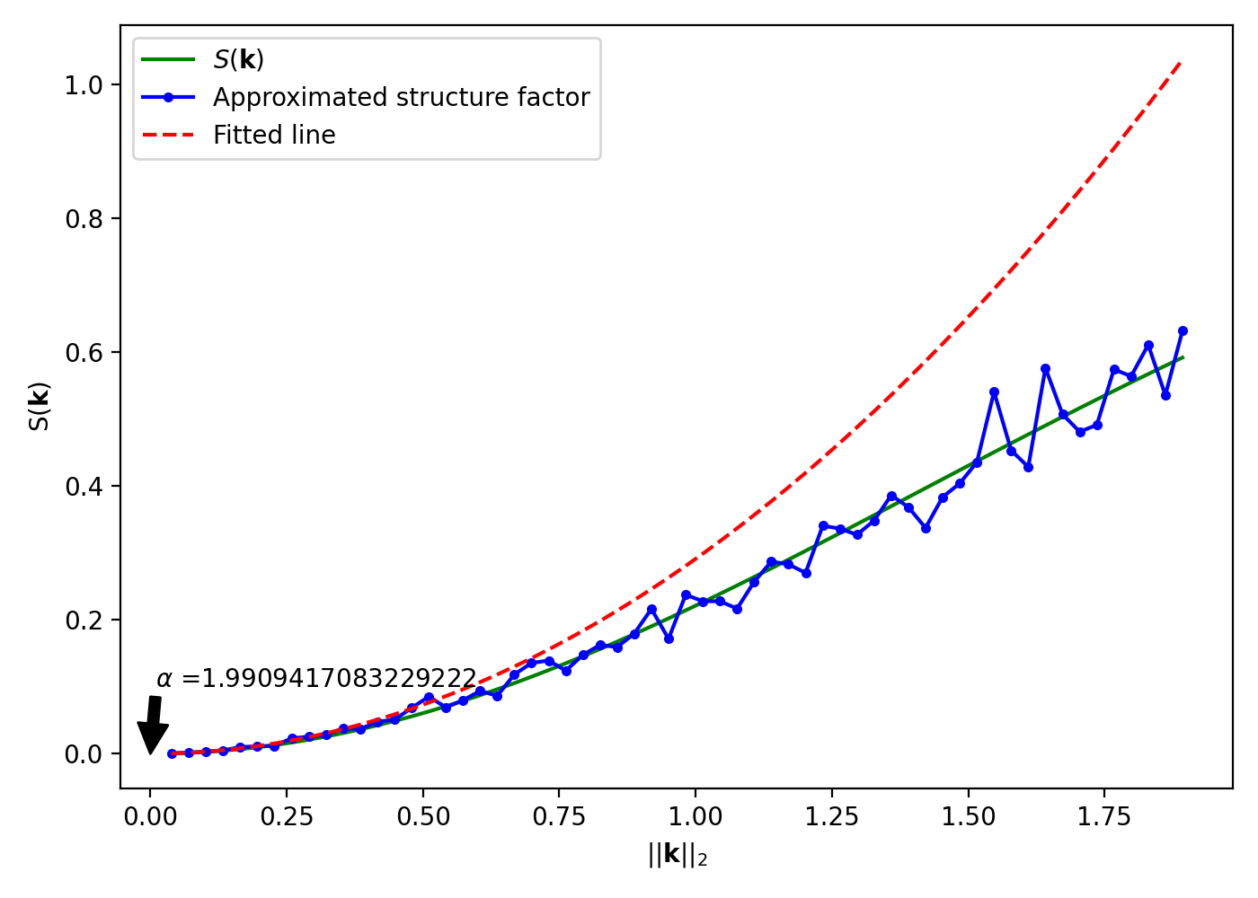
structure_factor.hyperuniformity.hyperuniformity_class(k_norm, sf, k_norm_stop=1, std_sf=None, **kwargs)[source]

Fit a polynomial \(y = c \cdot x^{\alpha}\) to sf around zero. \(\alpha\) is used to specify the possible class of hyperuniformity of the associated point process (as described below).

Parameters

k_norm (numpy.ndarray) – Vector of wavenumbers (i.e. norms of the wavevectors).
sf (numpy.ndarray) – Evaluations of the structure factor, of the given point process, at k_norm.
std (numpy.ndarray, optional) – Standard deviations associated to sf. Defaults to None.
k_norm_stop (float, optional) – Threshold on k_norm. The subvector obtained from sf starting from zero up to the value associated with k_norm_stop is used to fit a polynomial and find \(\alpha\). Defaults to 1.

Keyword Arguments

kwargs (dict) –

Keyword arguments (except “sigma”) of scipy.scipy.optimize.curve_fit parameters.

Returns

“alpha”: Estimated value of \(\alpha\).
”c”: Estimated value of \(c\).
”fitted_poly”: Polynomial used to find \(\alpha\).

Return type

dict(float, float, function)

Example

import matplotlib.pyplot as plt
from structure_factor.data import load_data
from structure_factor.hyperuniformity import hyperuniformity_class
from structure_factor.point_processes import GinibrePointProcess
from structure_factor.structure_factor import StructureFactor
from structure_factor.tapered_estimators_isotropic import (
    allowed_k_norm_bartlett_isotropic,
)

point_process = GinibrePointProcess()
point_pattern = load_data.load_ginibre()

sf = StructureFactor(point_pattern)
d, r = point_pattern.dimension, point_pattern.window.radius
k_norm = allowed_k_norm_bartlett_isotropic(dimension=d, radius=r, nb_values=60)
k_norm, sf_estimated = sf.bartlett_isotropic_estimator(k_norm)

summary = hyperuniformity_class(k_norm, sf_estimated, k_norm_stop=0.4)
sf_fitted_0 = summary["fitted_poly"](k_norm)

sf_theoretical = point_process.structure_factor(k_norm)

fig, ax = plt.subplots(figsize=(7, 5))
ax.plot(k_norm, sf_theoretical, "g", label=r"$S(\mathbf{k})$")
ax.plot(k_norm, sf_estimated, "b", marker=".", label="Approximated structure factor")
ax.plot(k_norm, sf_fitted_0, "r--", label="Fitted line")

ax.annotate(
    r"$\alpha$ ={}".format(summary["alpha"]),
    xy=(0, 0),
    xytext=(0.01, 0.1),
    arrowprops=dict(facecolor="black", shrink=0.0001),
)
ax.legend()
ax.set_xlabel(r"$||\mathbf{k}||_2$")
ax.set_ylabel(r"$\mathsf{S}(\mathbf{k})$")

plt.tight_layout(pad=1)

(Source code, png, hires.png, pdf)

Definition

For a stationary hyperuniform point process \(\mathcal{X} \subset \mathbb{R}^d\), if \(\vert S(\mathbf{k})\vert\sim c \Vert \mathbf{k} \Vert_2^\alpha\) in the neighborhood of zero, then by [Cos21] (Section 4.1.) the value of \(\alpha\) determines the hyperuniformity class of \(\mathcal{X}\) as follows,

Class	\(\alpha\)	\(\mathbb{V}\text{ar}\left[\mathcal{X}(B(0, R)) \right]\)
I	\(> 1\)	\(\mathcal{O}(R^{d-1})\)
II	\(= 1\)	\(\mathcal{O}(R^{d-1}\log(R))\)
III	\(]0, 1[\)	\(\mathcal{O}(R^{d-\alpha})\)

For more details, we refer to [HGBLachiezeR22], (Section 2.4).

Important

To compute \(\alpha\), a polynomial is fitted on the values of sf associated with a subvector of k_norm. This subvector is obtained by truncating k_norm around k_norm_stop. For the choice of k_norm_stop, the trade-off is to remain close to zero while including enough data points to fit a polynomial. In addition, std_sf will be considered while fitting the polynomial if it’s not None.

See also

StructureFactor
bin_data()
multiscale_test()
effective_hyperuniformity()

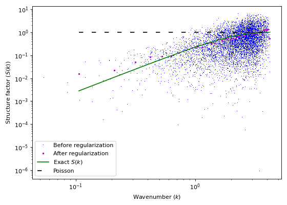
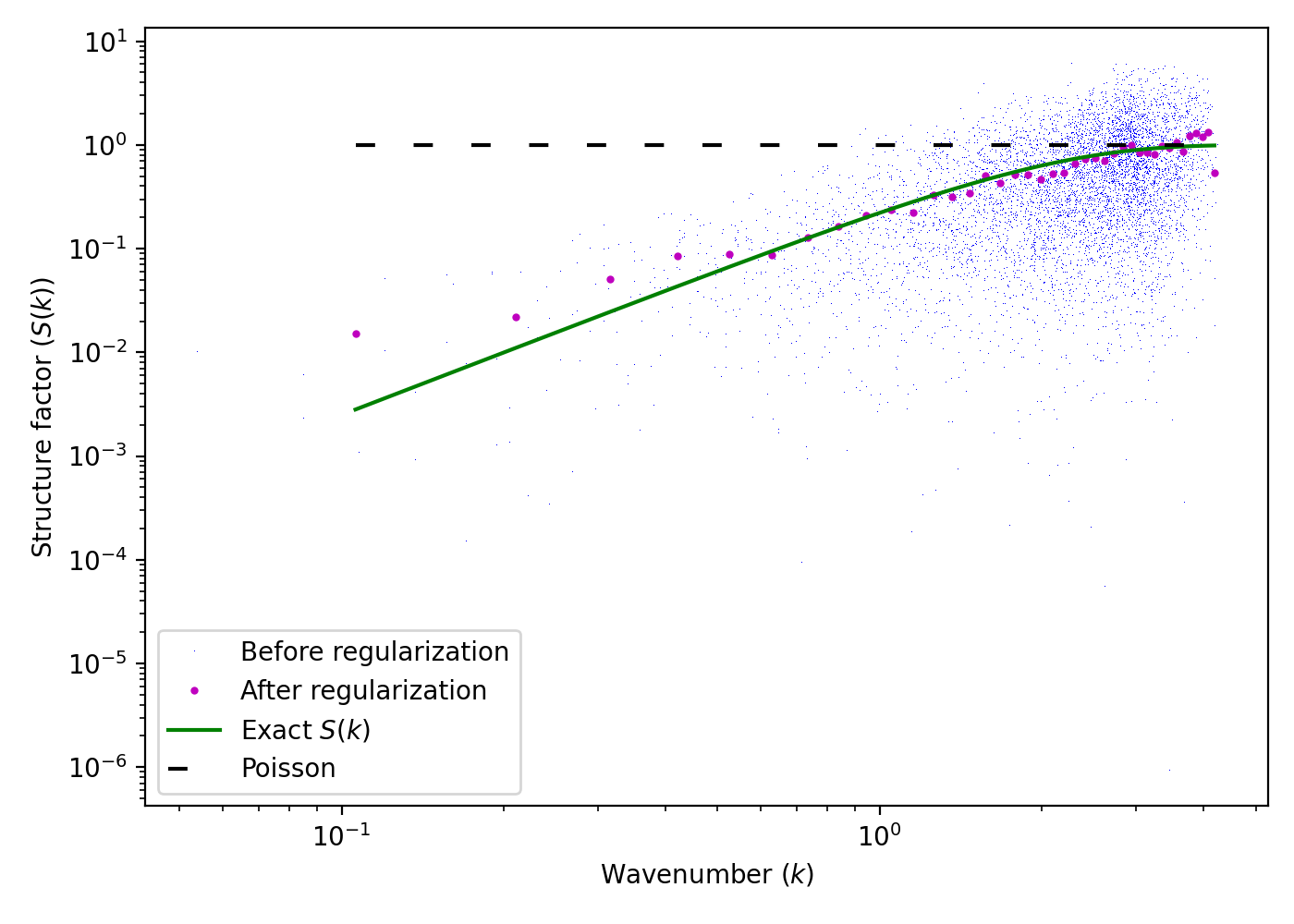
structure_factor.hyperuniformity.bin_data(k_norm, sf, **params)[source]

Split k_norm into sub-intervals (or bins) and evaluate, over each sub-interval, the mean and the standard deviation of the corresponding values in sf.

Parameters

k_norm (numpy.ndarray) – Vector of wavenumbers (i.e. norms of wavevectors).
sf (numpy.ndarray) – Evaluations of the structure factor, of the given point process, at k_norm.

Keyword Arguments

params (dict) – Keyword arguments (except “x”, “values” and “statistic”) of scipy.stats.binned_statistic.

Returns

k_norm: Centers of the bins.
sf: Means of the structure factor over the bins.
std_sf: Standard deviations of the structure factor over the bins.

Return type

tuple(numpy.ndarray, numpy.ndarray, numpy.ndarray)

Example

import matplotlib.pyplot as plt
import numpy as np
import structure_factor.utils as utils
from structure_factor.data import load_data
from structure_factor.hyperuniformity import bin_data
from structure_factor.point_processes import GinibrePointProcess
from structure_factor.spatial_windows import BoxWindow
from structure_factor.structure_factor import StructureFactor

point_pattern = load_data.load_ginibre()
point_process = GinibrePointProcess()

# Restrict point_pattern to window
window = BoxWindow([[-35, 35], [-35, 35]])
point_pattern_box = point_pattern.restrict_to_window(window)

# Estimate S
sf = StructureFactor(point_pattern_box)
x = np.linspace(0, 3, 80)
x = x[x != 0]
k = utils.meshgrid_to_column_matrix(np.meshgrid(x, x))
k, sf_estimated = sf.scattering_intensity(k)

# bin_data
k_norm = utils.norm(k)
k_norm_binned, sf_estimated_binned, _ = bin_data(k_norm, sf_estimated,bins=40)

fig, ax = plt.subplots(figsize=(7, 5))
ax.plot(k_norm, sf_estimated, "b,", label="Before regularization", rasterized=True)
sf.plot_isotropic_estimator(
    k_norm_binned,
    sf_estimated_binned,
    axis=ax,
    color="m",
    exact_sf=point_process.structure_factor,
    label="After regularization",
)
ax.legend()
plt.tight_layout(pad=1)

(Source code, png, hires.png, pdf)

Note

Typical usage

Regularize the results of StructureFactor to be used in effective_hyperuniformity() and hyperuniformity_class().

See also

StructureFactor

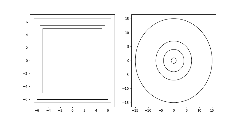
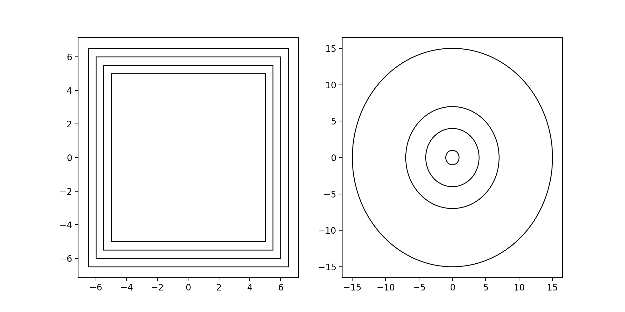
structure_factor.hyperuniformity.subwindows(window, subwindows_type='BoxWindow', param_0=None, param_max=None, params=None)[source]

Create a list of cubic (or ball)-shaped subwindows of a father window, with the associated minimum allowed wavevectors (or wavenumbers).

Parameters

window (AbstractSpatialWindow) – Father window.
subwindows_type (str, optional) – Type of the subwindows to be created. The available types are “BoxWindow” and “BallWindow”. The former for cubic and the latter for ball-shaped subwindows. Defaults to “BoxWindow”.
param_0 (float, optional) – Parameter (lengthside/radius) of the first subwindow to be created. If not None, an increasing sequence of subwindows with parameters of unit increments is created. The biggest subwindow has parameter param_max if it’s not None, else, the maximum possible parameter. Defaults to None.
param_max (float, optional) – Maximum subwindow parameter (lengthside/radius). Used when param_0 is not None. Defaults to None.
params (list, optional) – List of parameters (lengthside/radius) of the output subwindows. For a list of parameters of unit increments, param_0 and param_max can be used instead. Defaults to None.

Returns

subwindows: Obtained subwindows.
k: Minimum allowed wavevectors of allowed_k_scattering_intensity() or wavenumbers of allowed_k_norm_bartlett_isotropic() associated with the subwindow list. The former is for cubic and the latter for ball-shaped subwindows.

Return type

(list, list)

Example

from structure_factor.spatial_windows import BoxWindow
from structure_factor.hyperuniformity import subwindows

# Example 1: 
L = 30
window = BoxWindow([[-L / 2, L / 2]] * 2)
# subwindows and k
l_0 = 10
subwindows_box, k = subwindows(window, subwindows_type="BoxWindow", param_0=l_0)

# Example 2: 
subwindows_params=[1, 4, 7, 15]
subwindows_ball, k_norm = subwindows(window, subwindows_type="BallWindow", params=subwindows_params)

import matplotlib.pyplot as plt
fig, axis = plt.subplots(1, 2, figsize=(10,5))
axis[0].plot(0,0)
axis[1].plot(0,0)
for i, j in zip(subwindows_box, subwindows_ball):
    i.plot(axis=axis[0])
    j.plot(axis=axis[1])
plt.show()

(Source code, png, hires.png, pdf)

Note

Typical usage

Create the list of subwindows with the associated k to be used in multiscale_test().

See also